# starter code
library(RMariaDB)
library(DBI)
library(dbplyr)
library(tidyverse)
con_wai <- dbConnect(
  MariaDB(), host = "scidb.smith.edu",
  user = "waiuser", password = "smith_waiDB",
  dbname = "wai"
)
Measurements <- tbl(con_wai, "Measurements")
PI_Info <- tbl(con_wai, "PI_Info")
Subjects <- tbl(con_wai, "Subjects")

# collect(Measurements)Introduction
For this project, I am planning to recreate the Figure 1 graph from the National Library of Medicine. First, I am going to pull a dataset from SQL and read it into R to further manipulate and graph using ggplot. I plan on joining the Measurements dataset with the PI_Info dataset using their “Identifier” column and then using that new “ear_df” dataframe to select the specific information used in the original graph. From what I can see currently, the plot is a line-plot whose color is based on a combination of specific variables, so I will use that knowledge in my recreation. After the first half of the assignment is finished, I will further limit the data and create a new graph based on the “Age” variable from the Subjects dataset.
Reading in the Variables
SQL Code Creating a New Data Frame to Transport to R Environment
# Create a new data frame (ear_df) with specific variables based on a select few identifiers between a frequency of 200 and 8000
SELECT PI_Info.Year,
PI_Info.Identifier,
PI_Info.AuthorsShortList,
Measurements.Instrument,
Measurements.Frequency,
AVG(Measurements.Absorbance) AS Absorbance,
COUNT(DISTINCT SubjectNumber, Ear) AS Unique_Ears
FROM PI_Info
JOIN Measurements ON PI_Info.Identifier = Measurements.Identifier
WHERE PI_Info.Identifier IN ('Abur_2014', 'Feeney_2017',
'Groon_2015',
'Lewis_2015',
'Liu_2008',
'Rosowski_2012',
'Shahnaz_2006',
'Shaver_2013',
'Sun_2016',
'Voss_1994',
'Voss_2010',
'Werner_2010')
AND Frequency BETWEEN 200 AND 8000
GROUP BY Identifier, Instrument, Frequency
Graph Replication
# mutate the data frame to match the labels on the original graph
ear_df <- ear_df |>
  mutate(Instrument = if_else(Instrument == "Other", "not commerical system", Instrument)) |>
  mutate(legend = paste(AuthorsShortList, "(",Year,")", "N=", Unique_Ears,";", Instrument))
# recreate the original graph
ggplot(ear_df, aes(x = Frequency, y = Absorbance, color = legend)) +
  geom_line() +
  scale_x_log10() +
  scale_y_continuous(limits = c(0, 1)) +
  labs(
    x = "Frequency (Hz)",
    y = "Mean Absorbance",
    title = "Mean Absorbance from each publication in WAI database"
  )
Analysis of the Copied-Graph
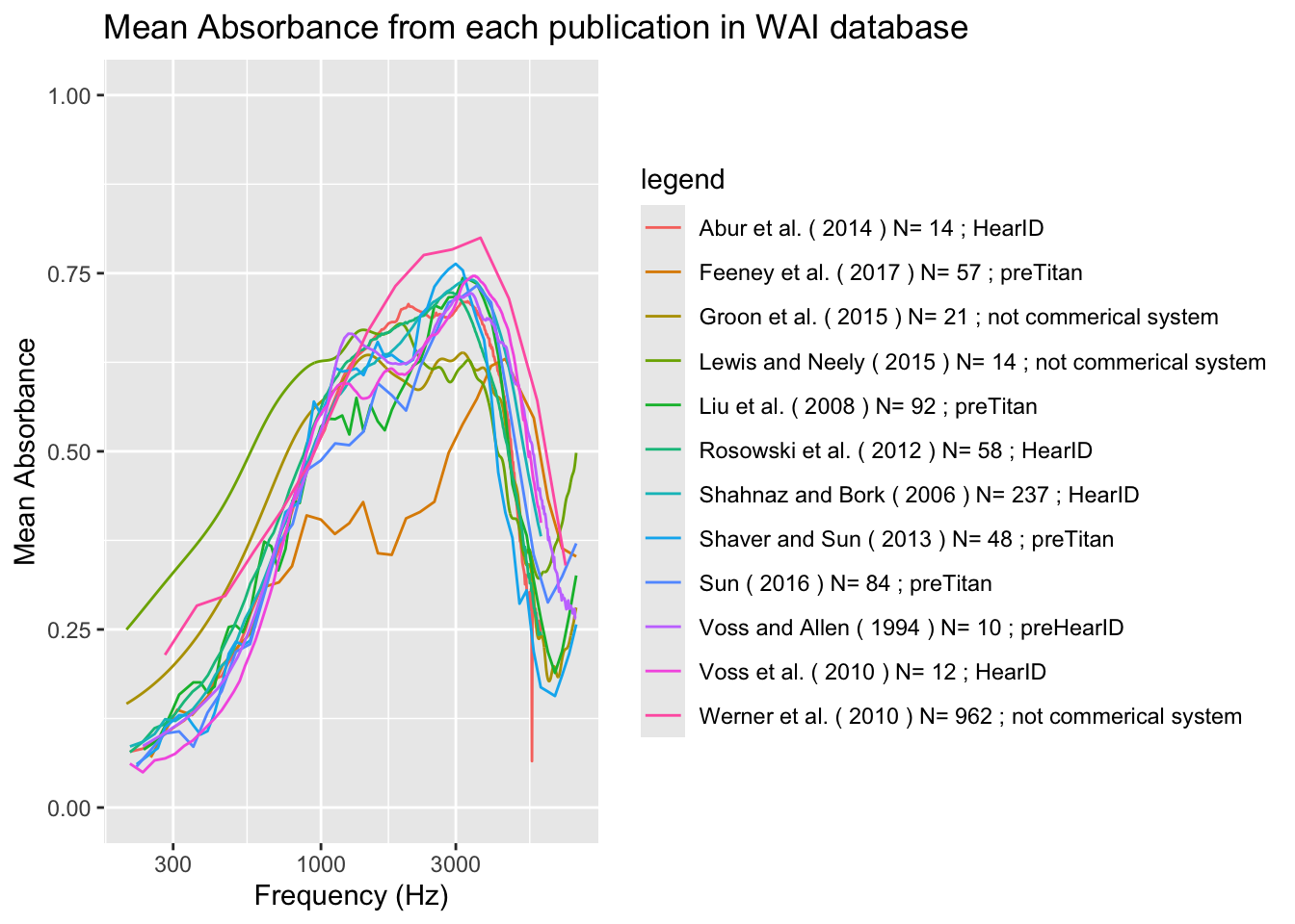
The graph above is a recreation (for the most part) of the Figure 1 plot I intended to copy. There are one or two datasets that are different from the original study, thus a perfect representation is most likely not possible using the data provided. This depicts the relationship between the mean absorbance (scaled from 0-1) and the frequency (with a range of 200-8000 Hz) based on a combination of variables. The legend explains the different lines of the graph, based on author, year, instrument used to conduct the experiment, and the number of “unique ears.” The peak is around 3000 Hz for most of the cases in the legend.
Further Analysis Based on Age
# select frequency, absorbance, and age to further analyze, saving as age_ear_df
SELECT Measurements.Frequency,
Measurements.Absorbance,
Subjects.AgeFirstMeasurement AS Age
FROM Measurements
JOIN Subjects ON Measurements.Identifier = Subjects.Identifier
WHERE Measurements.Frequency BETWEEN 200 and 8000
LIMIT 100000
Line Plot For Mean Absorbance Based on Age
# plot the relationship between frequency and absorbance based on age
ggplot(age_ear_df, aes(x = Frequency, y = Absorbance, color = Age)) +
  geom_line() +
  scale_x_log10() +
  scale_y_continuous(limits = c(0, 1)) +
  labs(
    x = "Frequency (Hz)",
    y = "Mean Absorbance",
    title = "Mean Absorbance from each publication in WAI database (By Age)"
  )
Analysis of Line Plot
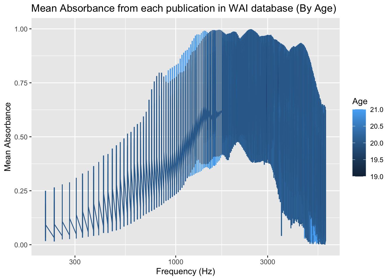
The above graph is very similar to the one already shown. The only difference for this specific plot is that the relationship between the mean absorbance (scaled from 0-1) and frequency (with a range of 200-8000 Hz) is based on the age of participants. The ages range from 19-21, including differences in ages based on half a year (i.e. 19.5, 20.5). Unlike the previous plot, there is no obvious peak, but rather an area (between 1000-6000 Hz) for the approximate max absorbance. There appears to not be a strong relationship based on the age; however, due to the difference being only two years, this would most likely have more significant results as the ages continue to increase. Note that the graph, although mostly accurate, is limited due to the restriction of the data to 100,000 in order for my computer to cooperate. With the full data, the graph may change slightly.
Conclusion
The concepts of my original plan were able to be executed; however, there were issues and a further depth of code than I originally accounted for, that was necessary to truly be successful in my plots. First, I had to individually limit, using the WHERE function, the “ear_df” data frame to the original twelve studies in the desired plot as well as the range of the Frequency variable. After that, the line plot was quite simple to recreate, but I had to scale the Y axis using the log10 function. Then, in the second half of the assignment, I made a new graph of Mean Absorbance and Frequency based on the Age variable in the Subjects data frame; however, due to the Subjects dataframe being extremely large, my computer was not loading after my attempt to join it with Measurements. After a while, I decided to limit the frame to 100,000 units and then the data frame had no problem producing in my Environment. I then made another line plot depicting this relationship.
Citation
I retrieved the original data from an article published by Susan E. Voss in the National Library of Medicine. The starter code comes from Johanna S. Hardin, a Pomona College professor of mathematics and statistics, for a mini-project in her Foundations of Data Science course.